
| 일 | 월 | 화 | 수 | 목 | 금 | 토 |
|---|---|---|---|---|---|---|
| 1 | 2 | 3 | ||||
| 4 | 5 | 6 | 7 | 8 | 9 | 10 |
| 11 | 12 | 13 | 14 | 15 | 16 | 17 |
| 18 | 19 | 20 | 21 | 22 | 23 | 24 |
| 25 | 26 | 27 | 28 | 29 | 30 | 31 |
- 그리디
- 구현
- 자료구조 및 실습
- test-helper
- cs
- docker
- 전산기초
- 프로그래머스
- 딥러닝
- AWS
- 파이썬
- CS231n
- Object detection
- C++
- 1단계
- 백준
- SWEA
- 이것이 코딩테스트다 with 파이썬
- ssd
- pytorch
- ubuntu
- 3단계
- 2단계
- 모두를 위한 딥러닝 강좌 시즌1
- Python
- 코드수행
- MySQL
- STL
- 실전알고리즘
- 머신러닝
- Today
- Total
곰퓨타의 SW 이야기
Lab 09-2 Weight initialization 본문
이 강의는 부스트코스에서 볼 수 있다!!
www.boostcourse.org/ai214/lecture/43760/
파이토치로 시작하는 딥러닝 기초
부스트코스 무료 강의
www.boostcourse.org
Why good initialization?
weight를 무작위로 초기화해서 무식하게 초기화했다!!
Geoffrey Hinton 교수님께서 말씀하신 것 중 일부분이다.
weight 초기화 방법을 적용한 것이 훨씬 더 학습이 잘 되고 성능이 뛰어나다는 것을 볼 수 있다.
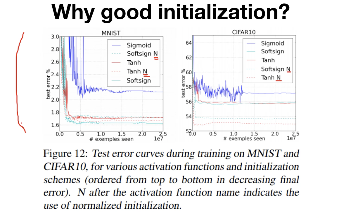
따라서 weight를 '잘' 초기화하는 것이 중요하다.
---> 어떻게 지혜롭게 initial weight value를 정할까??
- 상수로 초기화하기 (0으로 초기화하는 것은 좋지 않은 방식이다. backpropogation에서 gradient로 chain rule 적용할 때 weight가 0이면 학습이 어렵다.)
- 2006년 Hinton 교수님은 "A Fast Learning Algorithm for Deep Belief Nets"라는 논문을 통해 RBM(Restricted Boltzmann Machinne)이라는 것을 제시한다.
RBM/DBN
RBM (Restricted Boltzmann Machine) --> 1 layer
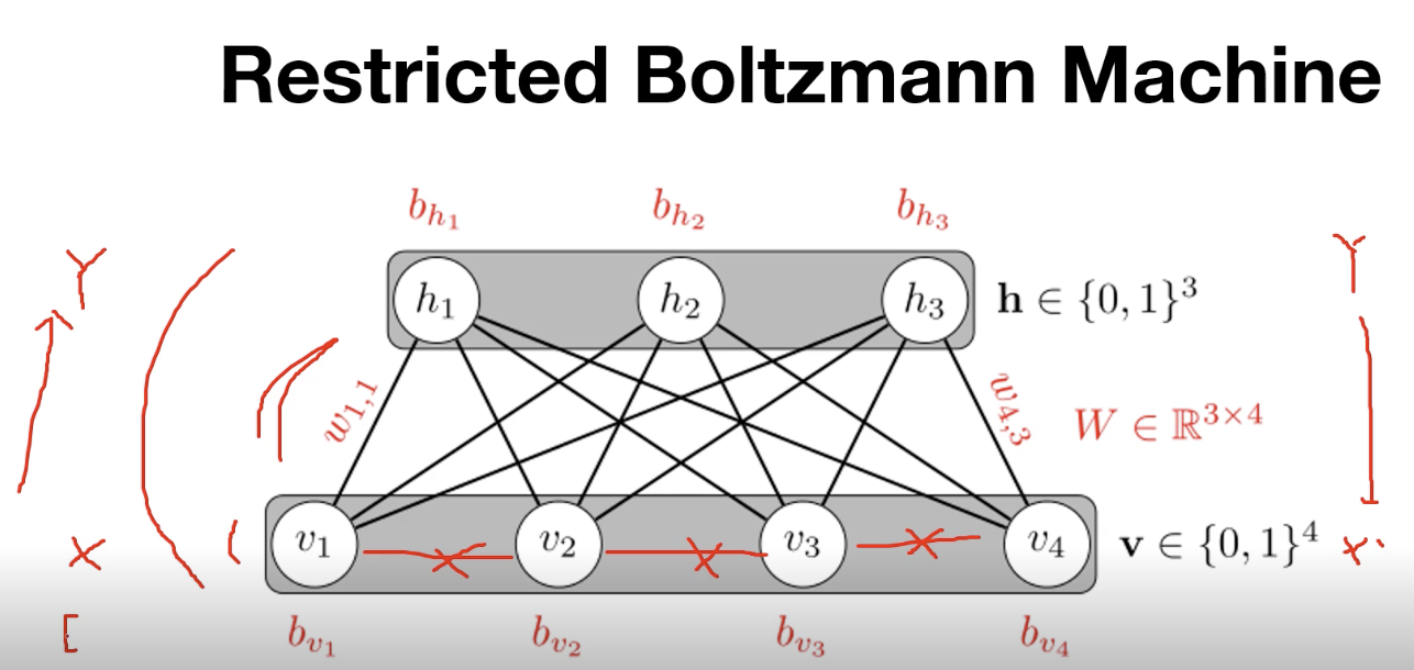
layer안에서는 연결이 없지만, 다른 layer 사이에 대해서는 fully connected 되어 있는 상태이다.
입력 X가 들어갔을 때 Y를 추출할 수 있고(encoding) Y가 들어갔을 때 X'을 도출할 수 있다(decoding).
RBM이 초기화하는 방법??
- 인접한 2개의 층을 pre-training step하였다. (X->Y , Y -> X')
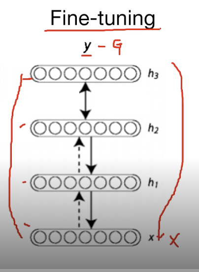
DBN : k개의 hidden layer 존재
- RBM 과정을 모든 layer에 대해 적용하여 stack과 같이 쌓으면서 전체 parameter를 업데이트한다.
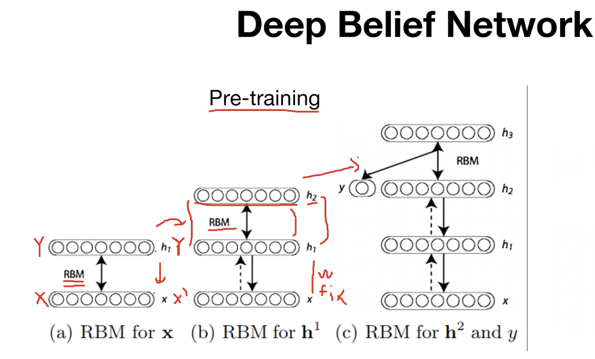
Pre-training이 완료되면 RBM으로 학습된 weight들이 있다.
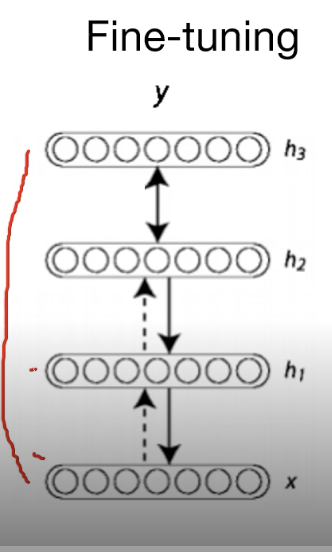
input X를 넣어 output Y를 도출하여 실제값 G와의 차이를 구하여(loss) backpropogation로 전체 network를 업데이트한다.
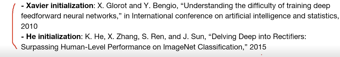
Xavier / He intialization (weight 초기화방법)
RBM 과정을 거치는 것이 아닌, 간단하게 초기화가 가능한 방법이다.
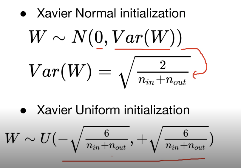
Xavier
- Xavier normal initialization
- Xavier Uniform initialization
layer마다 RBM을 적용했던 앞의 것과는 다르게, 수식에 집어넣어서 weight initialization을 하면 된다.
여기서 n_in은 input 개수이고 n_out은 output 개수이다.
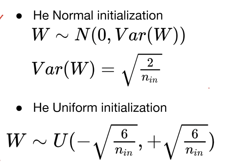
He initialization
- He initialization normal initialization
- He initialization Uniform initialization
Xavier에서 n_out이 없어진 형태라고 생각하면 된다!!
Code : mnist_nn_xavier
# https://pytorch.org/docs/stable/_modules/torch/nn/init.html#xavier_uniform_
def xavier_uniform_(tensor, gain=1.):
    # type: (Tensor, float) -> Tensor
    r"""Fills the input `Tensor` with values according to the method
    described in `Understanding the difficulty of training deep feedforward
    neural networks` - Glorot, X. & Bengio, Y. (2010), using a uniform
    distribution. The resulting tensor will have values sampled from
    :math:`\mathcal{U}(-a, a)` where

    .. math::
        a = \text{gain} \times \sqrt{\frac{6}{\text{fan\_in} + \text{fan\_out}}}

    Also known as Glorot initialization.

    Args:
        tensor: an n-dimensional `torch.Tensor`
        gain: an optional scaling factor

    Examples:
        >>> w = torch.empty(3, 5)
        >>> nn.init.xavier_uniform_(w, gain=nn.init.calculate_gain('relu'))
    """
    fan_in, fan_out = _calculate_fan_in_and_fan_out(tensor)
    std = gain * math.sqrt(2.0 / float(fan_in + fan_out))
    a = math.sqrt(3.0) * std  # Calculate uniform bounds from standard deviation

    return _no_grad_uniform_(tensor, -a, a)
pytorch를 이용하여 xavier로 weight을 초기화하는 방법은 다음과 같다.
xavier_uniform은 torch의 nn.init에 있다.
# xavier initialization
torch.nn.init.xavier_uniform_(linear1.weight)
torch.nn.init.xavier_uniform_(linear2.weight)
torch.nn.init.xavier_uniform_(linear3.weight)
weight 초기화 방식만 바꾸어도 정확도가 올라간다는 것을 알 수 있다!!
Code : mnist_nn_deep
좀 더 많은 linear를 쌓고, xavier를 사용한 경우이다.
# nn layers
# 최종 output을 제외하고 output을 512로 하였다.
# layer를 넓고 깊게 하였다.
linear1 = torch.nn.Linear(784, 512, bias=True)
linear2 = torch.nn.Linear(512, 512, bias=True)
linear3 = torch.nn.Linear(512, 512, bias=True)
linear4 = torch.nn.Linear(512, 512, bias=True)
linear5 = torch.nn.Linear(512, 10, bias=True)
relu = torch.nn.ReLU()


# xavier initialization
torch.nn.init.xavier_uniform_(linear1.weight)
torch.nn.init.xavier_uniform_(linear2.weight)
torch.nn.init.xavier_uniform_(linear3.weight)
torch.nn.init.xavier_uniform_(linear4.weight)
torch.nn.init.xavier_uniform_(linear5.weight)
이또한, 학습이 잘 되는 것을 확인할 수 있다.
'인공지능 > 부스트코스_파이토치로 시작하는 딥러닝 기초' 카테고리의 다른 글
| Lab 09-4 Batch Normalization (0) | 2021.02.26 |
|---|---|
| Lab 09-3 Dropout (0) | 2021.02.25 |
| Lab 09-1 ReLU (0) | 2021.02.25 |
| Lab 08-2 Multi layer Perceptron (0) | 2021.02.22 |
| Lab 08-1 Perceptron (0) | 2021.02.22 |


