
Notice
Recent Posts
Recent Comments
Link
| 일 | 월 | 화 | 수 | 목 | 금 | 토 |
|---|---|---|---|---|---|---|
| 1 | 2 | 3 | ||||
| 4 | 5 | 6 | 7 | 8 | 9 | 10 |
| 11 | 12 | 13 | 14 | 15 | 16 | 17 |
| 18 | 19 | 20 | 21 | 22 | 23 | 24 |
| 25 | 26 | 27 | 28 | 29 | 30 | 31 |
Tags
- 전산기초
- 프로그래머스
- pytorch
- Object detection
- 코드수행
- 이것이 코딩테스트다 with 파이썬
- 구현
- 머신러닝
- test-helper
- 파이썬
- Python
- 자료구조 및 실습
- MySQL
- 그리디
- 2단계
- SWEA
- CS231n
- C++
- AWS
- 모두를 위한 딥러닝 강좌 시즌1
- STL
- 백준
- 딥러닝
- 1단계
- ubuntu
- 3단계
- 실전알고리즘
- cs
- docker
- ssd
Archives
- Today
- Total
곰퓨타의 SW 이야기
Lab 08-2 Multi layer Perceptron 본문
이번에도 부스트코스의 강의를 참고하였다!!
www.boostcourse.org/ai214/lecture/43758/
파이토치로 시작하는 딥러닝 기초
부스트코스 무료 강의
www.boostcourse.org
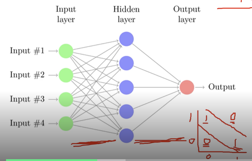
Multi layer Perceptron
1969년 Marvin Minsky는 XOR를 해결하기 위해 하나의 layer로는 해결할 수 없다고 하며 multilayer 개념을 설명하였다.
이는 여러 개의 층을 갖는 것으로, 선을 더 그어서 문제를 해결할 수 있도록 한다. =-> XOR 가능
하지만 그 당시에는 MLP를 학습시킬 수 있는 방법이 없었다. 이는 현재 backpropogation방법으로 해결할 수 있게 되었다.
Backpropogation
어떤 입력 X가 들어왔을 때 Y와 output의 차이를 loss라고 부르는데, loss에 대해서 W로 미분하여 loss 값을 최소화할 수 있는 방법을 고안한다. (이는 모두를 위한 딥러닝 강의 시즌 1 강의를 참고하라 하였다.. 이번주 안에 모두다 듣는 것이 목표이다...😂)
( https://www.youtube.com/watch?v=573EZkzfnZ0&feature=youtu.be 를 참고하면 된다!!)
X = torch.FloatTensor([[0, 0], [0, 1], [1, 0], [1, 1]]).to(device)
Y = torch.FloatTensor([[0], [1], [1], [0]]).to(device)


device = 'cuda' if torch.cuda.is_available() else 'cpu'

# for reproducibility
torch.manual_seed(777)
if device == 'cuda':
    torch.cuda.manual_seed_all(777)


w1 = torch.Tensor(2,2).to(device)
b1 = torch.Tensor(2).to(device)
w2 = torch.Tensor(2,1).to(device)
b2 = torch.Tensor(1).to(device)

def sigmoid(x) :
    return 1.0 / (1.0+torch.exp(-x))
    # return torch.div(torch.tensor(1), torch.add(torch.tensor(1.0),torch.exp(-x)))


def sigmoid_prime(x) :
    # sigmoid를 미분
    return sigmoid(x) * (1-sigmoid(x))


learning_rate = 1
for step in range(10001) :
    # forward
    l1 = torch.add(torch.matmul(X,w1),b1)
    a1 = sigmoid(l1)
    l2 = torch.add(torch.matmul(a1,w2),b2)
    Y_pred = sigmoid(l2)
    # binary cross entropy loss
    cost = -torch.mean(Y * torch.log(Y_pred) + (1-Y) * torch.log(1-Y_pred))


    # Backprop(chain rule)
    # loss derivative
    # 0으로 나누어지는 경우를 방지하기 위해 + 1e - 7
    d_Y_pred = (Y_pred - Y) / (Y_pred*(1.0 - Y_pred) + 1e-7)

    # layer 2
    d_l2 = d_Y_pred * sigmoid_prime(l2)
    d_b2 = d_l2
    # transpose : 2번째와 3번째 인자에 있는 것을 swap 시켜라
    # shape(10,5) 였다면 (5,10)이 된다.
    d_w2 = torch.matmul(torch.transpose(a1,0,1),d_b2)


    # layer 1
    d_a1 = torch.matmul(d_b2, torch.transpose(w2,0,1))
    d_l1 = d_a1 * sigmoid_prime(l1)
    d_b1= d_l1
    d_w1 = torch.matmul(torch.transpose(X,0,1),d_b1)


    # Weight update
    # 기존 weight에 backpropogation으로 구한 값과 learning rate의 곱을 빼준다.
    # gradient descent이므로 '-' 연산 수행
    # gradient ascent를 수행하고 싶다면 '+' 연산 수행
    w1 = w1 - learning_rate * d_w1
    b1 = b1 - learning_rate * torch.mean(d_b1,0)
    w2 = w2 - learning_rate * d_w2
    b2 = b2 - learning_rate * torch.mean(d_b2,0)

    if step % 100 == 0:
        print(step, cost.item())
Code : xor-nn
# Lab 9 XOR
import torch

device = 'cuda' if torch.cuda.is_available() else 'cpu'

# for reproducibility
torch.manual_seed(777)
if device == 'cuda':
    torch.cuda.manual_seed_all(777)


X = torch.FloatTensor([[0, 0], [0, 1], [1, 0], [1, 1]]).to(device)
Y = torch.FloatTensor([[0], [1], [1], [0]]).to(device)

# nn layers
# 2개의 layer를 가지는 multilayer perceptron(MLP)
linear1 = torch.nn.Linear(2, 2, bias=True)
linear2 = torch.nn.Linear(2, 1, bias=True)
sigmoid = torch.nn.Sigmoid()

# model
model = torch.nn.Sequential(linear1, sigmoid, linear2, sigmoid).to(device)

# pytorch에서 제공하는 것들 사용
# define cost/loss & optimizer
# binary cross entropy
criterion = torch.nn.BCELoss().to(device)
optimizer = torch.optim.SGD(model.parameters(), lr=1)  # modified learning rate from 0.1 to 1


for step in range(10001):
    optimizer.zero_grad()
    hypothesis = model(X)

    # cost/loss function
    cost = criterion(hypothesis, Y)
    cost.backward()
    optimizer.step()

    # 갈수록 loss가 줄어든다.
    if step % 100 == 0:
        print(step, cost.item())


# Accuracy computation
# True if hypothesis>0.5 else False
# 정확도 구하기
with torch.no_grad():
    hypothesis = model(X)
    predicted = (hypothesis > 0.5).float()
    accuracy = (predicted == Y).float().mean()
    print('\nHypothesis: ', hypothesis.detach().cpu().numpy(), '\nCorrect: ', predicted.detach().cpu().numpy(), '\nAccuracy: ', accuracy.item())
Code : xor-nn-wide-deep
4개의 layer를 쌓은 예시이다.
--> loss값이 조금 더 작게 학습되었다!
# Lab 9 XOR
import torch


device = 'cuda' if torch.cuda.is_available() else 'cpu'

# for reproducibility
torch.manual_seed(777)
if device == 'cuda':
    torch.cuda.manual_seed_all(777)


X = torch.FloatTensor([[0, 0], [0, 1], [1, 0], [1, 1]]).to(device)
Y = torch.FloatTensor([[0], [1], [1], [0]]).to(device)

# nn layers
# layer를 더 쌓음
# 이 예시에서는 4개짜리 MLP 생성함
linear1 = torch.nn.Linear(2, 10, bias=True)
linear2 = torch.nn.Linear(10, 10, bias=True)
linear3 = torch.nn.Linear(10, 10, bias=True)
linear4 = torch.nn.Linear(10, 1, bias=True)
sigmoid = torch.nn.Sigmoid()


# model
model = torch.nn.Sequential(linear1, sigmoid, linear2, sigmoid, linear3, sigmoid, linear4, sigmoid).to(device)


# define cost/loss & optimizer
criterion = torch.nn.BCELoss().to(device)
optimizer = torch.optim.SGD(model.parameters(), lr=1)  # modified learning rate from 0.1 to 1


# training
for step in range(10001):
    optimizer.zero_grad()
    hypothesis = model(X)

    # cost/loss function
    cost = criterion(hypothesis, Y)
    cost.backward()
    optimizer.step()

    if step % 100 == 0:
        print(step, cost.item())


# 정확도 측정
# Accuracy computation
# True if hypothesis>0.5 else False
with torch.no_grad():
    hypothesis = model(X)
    predicted = (hypothesis > 0.5).float()
    accuracy = (predicted == Y).float().mean()
print('\nHypothesis: ', hypothesis.detach().cpu().numpy(), '\nCorrect: ', predicted.detach().cpu().numpy(), '\nAccuracy: ', accuracy.item())'인공지능 > 부스트코스_파이토치로 시작하는 딥러닝 기초' 카테고리의 다른 글
| Lab 09-2 Weight initialization (0) | 2021.02.25 |
|---|---|
| Lab 09-1 ReLU (0) | 2021.02.25 |
| Lab 08-1 Perceptron (0) | 2021.02.22 |
| Lab 07-2 MNIST Introduction (0) | 2021.02.22 |
| Lab 07-1 Tips (0) | 2021.02.17 |
'인공지능/부스트코스_파이토치로 시작하는 딥러닝 기초' Related Articles
more


Comments