
| 일 | 월 | 화 | 수 | 목 | 금 | 토 |
|---|---|---|---|---|---|---|
| 1 | 2 | 3 | ||||
| 4 | 5 | 6 | 7 | 8 | 9 | 10 |
| 11 | 12 | 13 | 14 | 15 | 16 | 17 |
| 18 | 19 | 20 | 21 | 22 | 23 | 24 |
| 25 | 26 | 27 | 28 | 29 | 30 | 31 |
- ssd
- 모두를 위한 딥러닝 강좌 시즌1
- 파이썬
- docker
- MySQL
- C++
- ubuntu
- 딥러닝
- 전산기초
- 이것이 코딩테스트다 with 파이썬
- 프로그래머스
- test-helper
- 3단계
- 자료구조 및 실습
- AWS
- 구현
- SWEA
- CS231n
- 코드수행
- 백준
- cs
- 실전알고리즘
- STL
- 1단계
- 2단계
- Object detection
- Python
- 그리디
- 머신러닝
- pytorch
- Today
- Total
곰퓨타의 SW 이야기
Lab 09-1 ReLU 본문
이 강의를 참고하였다!!
www.boostcourse.org/ai214/lecture/43759/
파이토치로 시작하는 딥러닝 기초
부스트코스 무료 강의
www.boostcourse.org
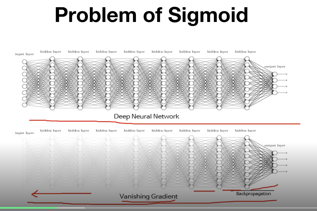
Problem of Sigmoid
input -> network -> output
( w ) ( loss 구하기)
<-----------------------backpropogation으로 weight 업데이트
sigmoid함수는 다음 사진과 같이 생겼는데, 양 끝쪽에서 문제가 생긴다.
backpropogation으로 gradient를 곱하게 되는데, 양끝에서 gradient가 0.xx와 같이 0에 가까운 숫자가 곱해지므로, vanishing 현상이 나타난다.
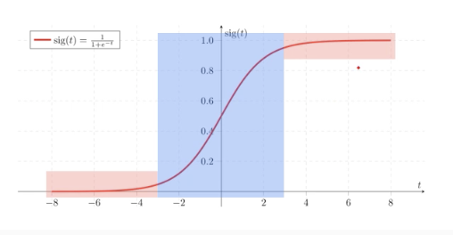
여러 개의 layer가 쌓이면 뒤에서는 gradient가 잘 전달이 되지만, 앞단으로 갈수록 gradient가 소멸하는 문제가 발생할 수 있다.
ReLU
f(x) = max(0,x)
그래프는 다음과 같은 그림을 갖는다.
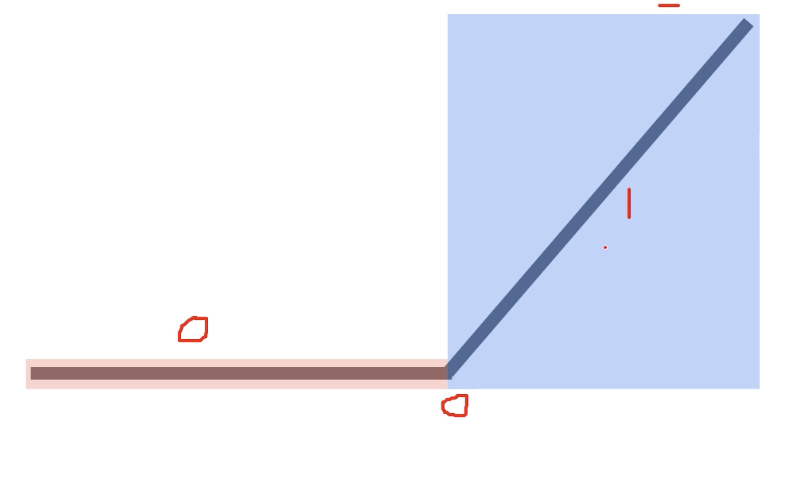
0이하에서는 gradient가 0이고, 0이후는 gradient가 1이되면서, 클수록 gradient가 0.xx되면서 사라지는 것을 보완할 수 있다.
하지만 음수 영역에서는 gradient가 0이기 때문에 음수 activation에서는 gradient가 사라지는 문제가 있다!
ReLU는 성능을 크게 향상시키는 데에 기여했다!!
코드로 작성하면 다음과 같다.
# torch에서 sigmoid를 사용할 때
x = torch.nn.sigmoid(x)

# torch에서 relu를 사용할 때
x = torch.nn.relu(x)

# 이 외의 activation function
torch.nn.tanh(x)
torch.nn.leaky_relu(x,0.01) # relu에서 음의영역에서 0만 넣는 것을 변형한 것이다.
Optimizer in PyTorch
torch.optim을 봄면 다양한 optimization algorithm이 구현되어 있다. 자주 사용하는 것들로는 다음과 같은 것이 있다.
torch.optim.SGD
torch.optim.Adadelta
torch.optim.Adagrad
torch.optim.SparseAdam
torch.optim.Adamax
torch.optim.ASGD
torch.optim.LBFGS
torch.optim.RMSprop
torch.optim.Rprop
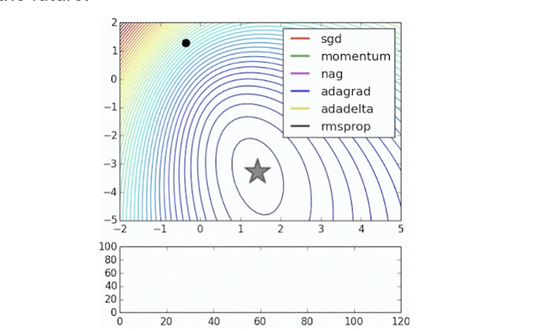
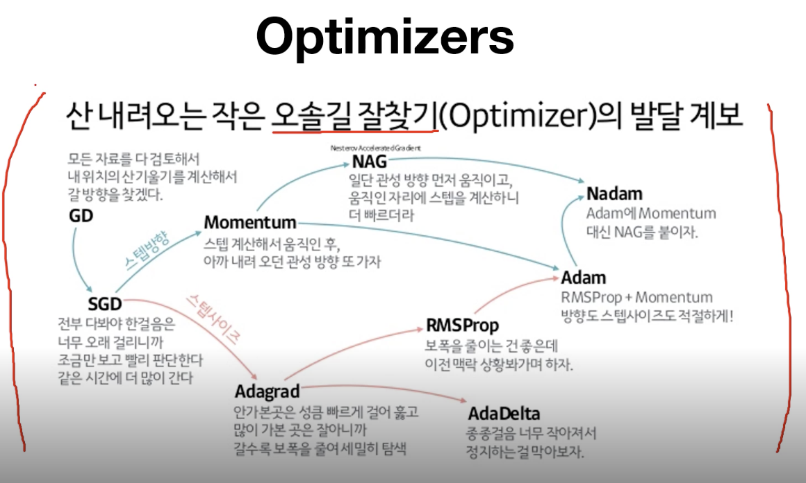
이는 학습을 진행하면서 각 optimizer가 어떻게 해를 찾아가는지 보여주는 그림이다.
다음은 오솔길을 찾는 것을 optimizer가 해야한다고 했을 때 어떤 전략으로 각각의 optimizer가 길을 찾는지 정리해놓은 것이다.
Review : reading data(MNIST)
# Lab 10 MNIST and softmax
import torch
import torchvision.datasets as dsets # dataset을 읽기 위한 dataset package
import torchvision.transforms as transforms
import random

# MNIST dataset
# train : train set을 불러올지 test set을 불러올지
# transform : 어떤 transform은 어떤 것을 적용할지
mnist_train = dsets.MNIST(root='MNIST_data/',
                          train=True,
                          transform=transforms.ToTensor(),
                          download=True)

mnist_test = dsets.MNIST(root='MNIST_data/',
                         train=False,
                         transform=transforms.ToTensor(),
                         download=True)


# dataset loader
# dataset : 어떤 데이터를 불러올지
# drop_last : 마지막 batch를 버릴지 말지
data_loader = torch.utils.data.DataLoader(dataset=mnist_train,
                                          batch_size=batch_size,
                                          shuffle=True,
                                          drop_last=True)


for epoch in range(training_epochs) :
	''
    for X,Y in data_loader:
    	X = X.view(-1,28*28).to(device)
Code : mnist 1 층의 layer
Softmax
# parameters 설정
learning_rate = 0.001
training_epochs = 15
batch_size = 100


# MNIST data image of shape 28 * 28 = 784
# 입력 개수, 출력개수(0-9까지의 class가짐) , bias
linear = torch.nn.Linear(784, 10, bias=True).to(device)


# Initialization
# weight를 normal distribution으로 초기화
torch.nn.init.normal_(linear.weight)


# define cost/loss & optimizer
# cross entropy loss 정의
criterion = torch.nn.CrossEntropyLoss().to(device)    # Softmax is internally computed.

# 이부분이 다름, SGD를 사용했었는데 다양한 optimization 중 Adam을 사용함
optimizer = torch.optim.Adam(linear.parameters(), lr=learning_rate)
Train
total_batch = len(data_loader)
for epoch in range(training_epochs):
    avg_cost = 0

    # X : data
    # Y : label
    for X, Y in data_loader:
        # reshape input image into [batch_size by 784]
        # label is not one-hot encoded
        X = X.view(-1, 28 * 28).to(device)
        Y = Y.to(device)

		# gradient 구하기
        optimizer.zero_grad()
        # 예측값
        hypothesis = linear(X)
        # 예측값과 실제값의 cost 구하기
        cost = criterion(hypothesis, Y)
        # backpropogation
        cost.backward()
        optimizer.step()

        avg_cost += cost / total_batch

    print('Epoch:', '%04d' % (epoch + 1), 'cost =', '{:.9f}'.format(avg_cost))

print('Learning finished')
Test
# Test the model using test sets
with torch.no_grad():
    X_test = mnist_test.test_data.view(-1, 28 * 28).float().to(device)
    Y_test = mnist_test.test_labels.to(device)

    prediction = linear(X_test)
    correct_prediction = torch.argmax(prediction, 1) == Y_test
    accuracy = correct_prediction.float().mean()
    print('Accuracy:', accuracy.item())

    # Get one and predict
    r = random.randint(0, len(mnist_test) - 1)
    X_single_data = mnist_test.test_data[r:r + 1].view(-1, 28 * 28).float().to(device)
    Y_single_data = mnist_test.test_labels[r:r + 1].to(device)

    print('Label: ', Y_single_data.item())
    single_prediction = linear(X_single_data)
    print('Prediction: ', torch.argmax(single_prediction, 1).item())
Code : mnist_nn 3층의 layer
# Lab 10 MNIST and softmax
import torch
import torchvision.datasets as dsets
import torchvision.transforms as transforms
import random


device = 'cuda' if torch.cuda.is_available() else 'cpu'

# for reproducibility
random.seed(111)
torch.manual_seed(777)
if device == 'cuda':
    torch.cuda.manual_seed_all(777)


# parameters
learning_rate = 0.001
training_epochs = 15
batch_size = 100


# MNIST dataset
mnist_train = dsets.MNIST(root='MNIST_data/',
                          train=True,
                          transform=transforms.ToTensor(),
                          download=True)

mnist_test = dsets.MNIST(root='MNIST_data/',
                         train=False,
                         transform=transforms.ToTensor(),
                         download=True)


# dataset loader
data_loader = torch.utils.data.DataLoader(dataset=mnist_train,
                                          batch_size=batch_size,
                                          shuffle=True,
                                          drop_last=True)


# nn layers
# 층수를 늘림 (깊게 쌓음)
linear1 = torch.nn.Linear(784, 256, bias=True)
linear2 = torch.nn.Linear(256, 256, bias=True)
linear3 = torch.nn.Linear(256, 10, bias=True)
# relu activation function 사용
relu = torch.nn.ReLU()


# Initialization
# 각 weight 값 초기화
torch.nn.init.normal_(linear1.weight)
torch.nn.init.normal_(linear2.weight)
torch.nn.init.normal_(linear3.weight)


# model
# 층 모델
# 마지막 layer에서는 relu를 적용하지 않은 이유 :
#          cross entropy를 사용할 것이므로 softmax로 dimension 해주어야 한다.
# -->별도의 activation을 설정하지 않았다.
model = torch.nn.Sequential(linear1, relu, linear2, relu, linear3).to(device)


# define cost/loss & optimizer
criterion = torch.nn.CrossEntropyLoss().to(device)    # Softmax is internally computed.
optimizer = torch.optim.Adam(model.parameters(), lr=learning_rate)


'''
Train
'''
total_batch = len(data_loader)
for epoch in range(training_epochs):
    avg_cost = 0

    for X, Y in data_loader:
        # reshape input image into [batch_size by 784]
        # label is not one-hot encoded
        X = X.view(-1, 28 * 28).to(device)
        Y = Y.to(device)

        optimizer.zero_grad()
        hypothesis = model(X)
        cost = criterion(hypothesis, Y)
        cost.backward()
        optimizer.step()

        avg_cost += cost / total_batch

    print('Epoch:', '%04d' % (epoch + 1), 'cost =', '{:.9f}'.format(avg_cost))

print('Learning finished')


'''
Test
'''
# Test the model using test sets
# 1개를 사용했을 때보다 3개의 layer를 가지고 학습했을 때 더 좋은 성과를 냈다.
with torch.no_grad():
    X_test = mnist_test.test_data.view(-1, 28 * 28).float().to(device)
    Y_test = mnist_test.test_labels.to(device)

    prediction = model(X_test)
    correct_prediction = torch.argmax(prediction, 1) == Y_test
    accuracy = correct_prediction.float().mean()
    print('Accuracy:', accuracy.item())

    # Get one and predict
    r = random.randint(0, len(mnist_test) - 1)
    X_single_data = mnist_test.test_data[r:r + 1].view(-1, 28 * 28).float().to(device)
    Y_single_data = mnist_test.test_labels[r:r + 1].to(device)

    print('Label: ', Y_single_data.item())
    single_prediction = model(X_single_data)
    print('Prediction: ', torch.argmax(single_prediction, 1).item())
이러한 코드는 github.com/deeplearningzerotoall/PyTorch 에 더 자세히 나와있다!!
'인공지능 > 부스트코스_파이토치로 시작하는 딥러닝 기초' 카테고리의 다른 글
| Lab 09-3 Dropout (0) | 2021.02.25 |
|---|---|
| Lab 09-2 Weight initialization (0) | 2021.02.25 |
| Lab 08-2 Multi layer Perceptron (0) | 2021.02.22 |
| Lab 08-1 Perceptron (0) | 2021.02.22 |
| Lab 07-2 MNIST Introduction (0) | 2021.02.22 |


